Payment Curve (Part 3) – Alternate Payment Curves

In a previous post we looked at the common types of Payment Curves used in a Performance Based Contract (PBC). These were the All or None Payment Curves, Linear Payment Curves and the Non-Linear Payment Curves. In this post we are going to look at the more uncommon types of Payment Curves, or what my colleagues and I call the Alternative Payment Curves, including Demerit Point and Visual Payment Curves.

While not strictly a Payment Curve, the Demerit Point approach measures the total number of Demerit Points incurred during a Review Period and modifies Contractor Payment based on a performance assessment of each event. Where the event experiences reduced performance or non-performance, Demerit Points are awarded based on how significant/important the event is. For example, Table 1 highlights one approach to awarding the number of demerit points based on how significant/important the event is:

Demerit Point Table

Table 1: Demerit Point Evaluation

The total amount of Demerit Points incurred for all events in the Review Period is then used to calculate the payment. Figure 1 illustrates the corresponding Demerit Point Payment Curve for Table 1:

Payment Curve - Demerit Point

Figure 1: Demerit Point Payment Curve

If used appropriately, Demerit Point payment curves are very efficient when measuring contractor responsiveness to a variety of demands (e.g. urgent and routine) within the same performance measure.

Alternate Payment Curves – Visual

Unlike the other Payment Curves, the Visual Payment Method uses visual indicators (e.g. ‘dots’) to register satisfaction. This includes partial, of softer subjective measures such as customer satisfaction, quality of a meal, etc. This approach can combine many outcomes by using a number of ‘dots’. For example, increasing the number of ‘dots’ against a specific performance measure (e.g. quality of meal) highlights the relative importance of the area to the contractor. To calculate the APS as a percentage, compare the total number of ‘dots’ against the possible total of ‘dots’. Figure 2 illustrates a Visual Payment Curve:

Payment Curve - Visual

Figure 2: Visual Payment Curve


Posted in Basis of Payment, payment curve, the How | Tagged , , , , , | 1 Comment

Payment Curves (Part 2) – Common Performance Curves

In an earlier post we described the role and common features of a Payment Curve used in a Performance Based Contract (PBC), including the difference between Achieved Performance and the Adjusted Performance Score. In the first of two posts we will look at the 4 different types of Payment Curves that are commonly used in a PBC.  Specifically, there are 4 types of Payment Curves used in PBCs as follows:

  1. All or None Payment Curves
  2. Linear Payment Curves
  3. Non-Linear Payment Curves
  4. Alternative Payment Curves, including Demerit Point and Visual Payment Curves.

So let us look at each of these Payment Curves.

All or None Payment Curves

Simply put, if the required contracted level of performance is met the contractor gets 100% of their performance payment. However, if the required level of performance is not met the contractor gets 0% of their performance payment. This can be seen in Figure 1 noting the two charts in Figure 1 represent the two cases where (1) any decrease in achieved performance is worse to the seller, and where (2) an increase in achieved performance is worse.

This is typical of any Contract that has a Liquidated Damages (LD) clauses where poor performance, often in terms of a delay of delivery, results in the awarding of a pre-agreed genuine estimate of financial damages to the seller.

Payment Curve - All or None

Figure 2: All or None Payment Curve 

Liquidated Damages (LDs)

There is a common misunderstanding that a PBC approach that ties Contractor payment to performance replaces any need for Liquidated Damages (LDs). Where appropriate, LDs are included against traditional contract milestones, such as establishment of the Contractor support organisation (e.g. Operative Date (OD)).

However, LDs can also be used in combination with a PBC payment curve. LDs may be applied where there is no value to the seller in the level of service provided by the Contractor. As damage has occurred an alternative method for delivery of the services required must be considered.

Linear Payment Curves

Unlike the All or None Payment Curve, the Linear Payment Curve reduces payment based on a straight line between the Achieved Performance and variation from the contracted level. It should be noted that 0% Adjusted Performance does not have to occur at 0% Achieved Performance. Alternatively, this linear form can be represented through a series of equal steps. This can be seen in Figure 2.

Payment Curve - Linear

Figure 2: Linear Payment Curve

Non-Linear Payment Curves

Similar to the Linear Payment Curve, the Non-Linear Payment Curve reduces payment based on Achieved Performance variation from the contracted level. However, in this case the reduction in payment is represented by a curve, multiple linear sections, or an unequal series of steps. These variations can be seen in Figure 3.

Payment Curve - Non-Linear

Figure 3: Non-Linear Payment Curve

Posted in Basis of Payment, payment curve, the How | Tagged , , , , , | 2 Comments

Payment Curves (Part 1)

Changes to Contractor payments based on Contractor performance is one of the fundamental tenets of the Performance Based Contracting (PBC) approach. While changing payment uses a variety  of methods, all typically use a Payment Curve to describe how to change the payments. But, before we look at the different types of Payment Curves let’s look at the common features.

Figure 1 illustrates a generic Payment Curve based on the Support variant of the Australian Standard for Defence Contracting (ASDEFCON) series of contract templates used by the Australian Department of Defence.

Payment Curve

Figure 1: Australian Standard for Defence Contracting (ASDEFCON) Payment Curve

Before we look at the key features, it is important to note that each Key Performance Indicator (KPI), or payment performance measure, will have their own Payment Curve. For example, if your PBC had 3 KPIs you are likely to have 3 different Payment Curves.

Noting this, let’s examine some of the key features of a Payment Curve.

The most important feature is that there are 2 dimensions to the Payment Curve. Firstly, the horizontal axis or line, called Achieved Performance, and secondly the vertical axis or line, called the Adjusted Performance Score or APS. The overall intent of the Payment Curve is to change Contractor performance into Contractor payment.

The Achieved Performance represents the actual score that the Contractor reached for the particular Review Period. This could be for an individual event such as deeper maintenance; or over a period of time such as a month or a quarter. Importantly, the unit of measurement for the Achieved Performance reached reflects the unit of the relevant KPI and can represent time (e.g. hours, days, etc.), or other values (e.g. number of items, percentages, etc.)

In contrast, the APS is the percentage of Contractor payment linked to the KPI based on their corresponding Achieved Performance. The unit of APS is always a percentage. Accordingly, many practitioners consider the Payment Curve as a method of translating Achieved Performance to APS.

At the end of the Review Period (e.g. month, quarter, etc.), when determining the overall Weighted Performance Score (see Performance Measure Weighting) the Contractor’s Achieved Score for each KPI is calculated using the specific formula and business rules. The Review Period Achieved Score (in the units of the KPI, such as days) is then compared to the specific Payment Curve to calculate the APS as a percentage. Of course, your calculation may also include a Performance Measure Gate which was discussed in a earlier post.

Now we understand the role of a Payment Curve and the common features, in the next post, we will look at the 4 different types of Payment Curves that are commonly used in a PBC.

Posted in Basis of Payment, payment curve, the How | Tagged , , , , , | 2 Comments

Performance Measure Gate

One advanced, yet uncommon, approach to performance management in a Performance Based Contract (PBC) is the concept of a performance measure ‘gate’ which modifies the overall Weighted Performance Score (WPS) based on specific criteria.

A gate can be used where there is a critical requirement (typically safety or statutory/law) that must be met before making the final performance assessment. It may help to think of it as a pre-requisite before calculating the overall WPS.

The intent of using a gate is to make sure the contractor recognises that there are some underlying minimal performance requirements that must be met before considering the delivery of service. This can either be applied to an individual performance measure or the overall WPS. Given this minimal requirement these types of contracts are sometimes called a ‘safety before profit’ contract.

For example, consider a PBC that requires a contractor to deliver meals and their performance is measured (and paid) based on the timeliness of the meals, quality of the meals and the number of meal choices. However, it is also possible to include a ‘gate’ that modifies the overall WPS based on the number of confirmed cases of food poisoning. In this case, the use of a gate highlights to the contractor that if there is a choice between being on time with the meals and under-cooking them leading to food poisoning, the contractor should met the more important safety requirement and not simply be on time not that I am suggesting that this occurs!

So how does this work in practice? In calculating the overall WPS we place a gate as follows:

Final WPS = overall WPS x gate

where:
overall WPS = performance score for the period of observation for the overall WPS; and
gate = 1 or 0 , based on the defined conditions (e.g. confirmed case of food poisoning)

In our example, if the contractor got an overall WPS of 85% for the month, yet there was 1 confirmed case of food poisoning, then the overall WPS would be set to 0% for the month.

The above example highlights the main issue when using a gate and why they are rarely used. For example, given this “all or none” approach, if a gate is triggered on day 1 of the month and there is no possibility of getting any of the performance payment what financial motivation does the contractor have to perform for the rest of the month? Recognising this, options to address this include reducing this impact of the gate (e.g. not 0 or 1, but rather some significant reduction such as 0.5 or 50% which means the contractor cannot earned greater than 50% of the performance fee) or an ability to “earn back” some of this loss through either additional (value add) work or superior performance.

So while they are not common in PBCs it is important as PBC practitioners to consider whether (1) a gate could apply for your contract scope and the performance measures you have chosen and (2) if so, what it the effect when the gate is triggered.

Posted in Basis of Payment, Performance Measure, the How | Tagged , , , , , , | 1 Comment

Performance Measure Weighting

Up until now we have spoken about single performance measures. However, typically a Performance Based Contract (PBC) will use more than 1 performance measure. Therefore, the question is how do we amalgamate two or more performance measures into one overall Weighted Performance Score (WPS)?

Firstly, my colleagues and I define a WPS as a single number (typically a percentage) that represents the overall score of all performance measures used within the PBC. Typically the WPS is the value that is then applied to any form of payment.

In terms of the calculating the WPS there are two methods; (1) equally weighted or (2) unequally weighted. Additionally, the PBC practitioner can also add ‘gates’ into the WPS calculation, however, this is the topic of a future post.

Equally Weighted WPS

The equally weighted WPS is based on the following equation:

Screen Shot 2016-06-18 at 12.24.16 PM

Where

  • Total Score (%) of all PM = the sum of all performance measures (in the same units, typically percentage)
  • Number of PMs = the total number of performance measures

For example if we had a PBC with 3 performance measures with the performance scores for each performance measure in the last performance period being PM1 = 90%, PM2 = 80% and PM3 = 100% then the equally weighted WPS would be:

Screen Shot 2016-06-18 at 12.24.22 PM

The advantage of the equally weighted WPS is that it is simple to apply and easy to understand. However, the disadvantage of the equally weighted WPS is that it can mask under performance in a critical performance measure.

Unequally Weighted WPS

The unequally weighted WPS is based on the following equation:

Screen Shot 2016-06-18 at 12.24.29 PM

Where

  • Weighting PM = the weighting represented as a percentage (typically between 0% and 100%) for the individual performance measures
  • Score PM = the performance score of the individual performance measure for the last performance period

Using the same example as before, if we had a PBC with 3 performance measures with the performance scores for each performance measure being PM1 = 90%, PM2 = 80% and PM3 = 100%, however, in this case the weightings of the performance measures were PM Weight 1 = 50%, PM Weight 2 = 30% and PM Weight 3 = 20% then the unequally weighted WPS would be:

Screen Shot 2016-06-18 at 12.24.37 PM

The advantage of the unequally weighted WPS is that it is highlights to the seller the buyers performance priorities based on performance measure with the highest weighting. However, the disadvantage of the unequally weighted WPS is that it more complex to apply and harder to set the weightings

Critical to the successful operation of an unequally weighted WPS is setting the weightings. In establishing these weighting the designer must remember that the weightings reflect the relative importance of each performance measure over the other performance measures. For example, is performance measure 1 more (or less or equally) important as performance measure 2? If more important, how much more important? When establishing the unequal weightings the following rules of thumb should be observed:

  • Consider the relative values of weights to highlight priority (e.g. KPI-1 is twice as important as KPI-2)
  • Use only 5% increments (e.g. not 2.5 or less)

Again, considering the previous example where PM1 = 50% weighting, PM2 = 30% weighting and PM3 = 20% weighting we can determine that PM1 is more than 1.5 times more important than PM2 and more than 2 times more important than PM3. Based on this simple observation the PBC practitioner can then check with the buyer whether this accurately reflects their priorities.

In summary, while the calculation of the WPS is typically considered a minor element of the design of a PBC the use of weightings (or not) is a critical element in highly successful PBCs.

Posted in Performance Measure, the How | Tagged , , , , , , , , , , | 6 Comments

Availability in Performance Based Contracts – Part 2

In an earlier part (Availability Part 1) we described availability as one of the highest priorities of system or service performance in a Performance Based Contract (PBC). We defined is as:

“Availability – providing users with material / services that are in a known state and ready to meet operational preparedness requirements.”

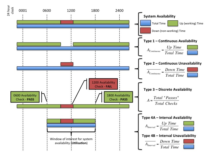
We then described availability performance measures using 4 types; Type 1 Continuous Availability, Type 2 Continuous Unavailability, Type 3 Discrete Availability and Type 4a Interval Availability / Type 4b Interval Unavailability.

While this is a good start we need to look at a some other considerations.

The first consideration is whether the measure represents availability of a number (or fleet) of systems, potentially in multiple geographic locations, or whether the measure only a single system. For example, if I need availability of a tower crane on two different construction sites, when designing the availability measure does the measure represent each site independently or combines both sites? The real question here is whether the measure represents the buyer’s requirement, in this case availability of a tower crane that on both sites to help the construction team. Having a tower crane available on the other construction site when needed on this site does not help. Therefore, care is needed when designing the availability performance measure to accurately reflect whether it represents a single system or fleet, and then how is it averaged (see earlier post on averaging), and potentially then amalgamated with other performance measures (see Weighting Performance Measures).

The second consideration of the measure is defining availability in terms of what sub-systems or components needs to work. For example, consider a complex piece of equipment such as a commercial passenger aircraft such as the Boeing 737. In the case of aircraft there is a minimum criteria of systems that must work for the aircraft to be considered available referred to as the Master Minimum Equipment List (MMEL).  The MMEL describes those sub-systems and equipment that for reasons of safety must be working (e.g. engines, control systems, life vests and rafts, etc.). However, the MMEL doesn’t include optional systems such as the entertainment system. So if the aircraft is safe to fly but the entertainment system isn’t working, is the aircraft available? Now this may be OK for a 1 hour flight, however, if you have ever flown 13 hours from Australia to the US, this is a very different question. Therefore, we need to carefully define what we mean by available in terms of the working order.

Additionally, we need to define any variation between fully functioning vs. partially functioning vs. not functioning. The United States Air Force (USAF) has a term to represent this:

  • Fully Mission Capable (FMC) reflecting the aircraft’s ability to undertake any mission without restriction to the user;
  • Not Mission Capability (NMC) reflecting the aircraft’s inability to undertake any mission regardless of restriction; and
  • Partially Mission Capable (PMC) reflecting the aircraft’s ability to only under a subset of the required missions thereby restricting operations to the user.

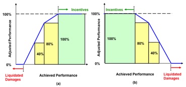
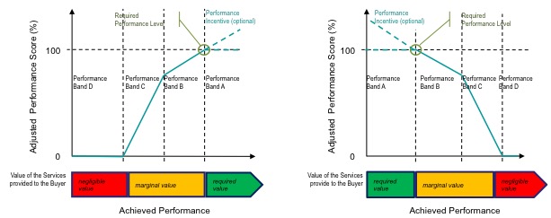
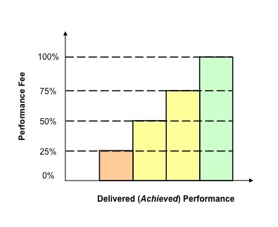
While this approach makes sense, the question is how do we score availability for each of these availability states? For example, is the score for FMC equal to PMC? If so, then how do we motivate the seller to deliver FMC rather than PMC every time? Alternatively, if PMC is equal to NMC then is the buyer missing out on availability that could be used? In many cases this situation is addressed by setting FMC to 1 (or 100%), NMC equal to 0 (or 0%) and PMC somewhere between 0.5 to 0.7 (or 50% to 70%) to represent potential benefits to the buyer if the seller offered a PMC aircraft, however, the buyer being clear that the benefits of PMC are not equal to FMC.

Finally, and as required for any performance measure, we need to define who takes the measurement, scores the availability and over what period (e.g. daily, weekly, monthly, quarterly, annually, etc.).

In summary, while availability performance measures represent the goal of many PBC buyers and sellers, care must be taken when designing these measures to ensure that they accurately reflect the need.

Posted in Performance Measure, the How | Tagged , , , , , , , | 1 Comment

Availability in Performance Based Contracts- Part 1

“Lost time is never found again.”

Benjamin Franklin

In Performance Based Contracting (PBC) considering availability of a system or service is one of the highest requirements and priorities for both buyer and seller. But what is availability and how do we describe it within our PBC?

Although we could use various definitions of availability such as those from the Reliability engineering field (e.g. US Military Standard 721C) my colleagues and I simply use the following definition as part of our Key Result Areas (KRAs) structure within our PBCs:

“Availability – Providing users with material / services that are in a known state and ready to meet operational preparedness requirements.”

While we have now defined availability creating an availability performance measure is slightly more complicated given our experience shows there are 4 types of availability performance measures. This variety is illustrated below using an example of a system whose availability can be automatically monitored.

Measuring Availability

Measuring Availability in a Performance Based Contract

Now lets consider each type of availability performance measure described in the diagram above.

Type 1 Continuous Availability – this type of measure simply compares the amount of working (operational) time vs. total time across a certain review period such as a day (24 hours), week or month. This is a standard measure used by mobile telephone companies, Internet Service Providers, cable / satellite TV companies, etc. where the continuous availability of their service is key to their success. A type 1 availability performance measure is typically represented as a percentage.

Type 2 Continuous Unavailability – where the performance level of the availability is very high (e.g. 99.9996%) it may be simpler to define the amount of unavailability allowed. A type 2 availability performance measure is typically expressed as an amount of time (e.g. 2 hours downtime per month).

Type 3 Discrete Availability – unlike a type 1 or 2 availability performance measure a type 3 does not measure availability continuously. Instead it uses at least 1, possibly more, points in time that defines when to measure availability of the system. For example, it could measure availability at the start of each day / shift. Or it may measure every 3 or 6 hours. The typical reason for the variation from a type 1 / 2 measure is that the continuous measurement of availability may not be possible for some systems or the cost of continuously collecting availability data could be too high. A type 3 availability performance measure can be represented either as a percentage or as a state (e.g. pass / fail).

Type 4a Interval Availability / Type 4b Interval Unavailability – while very similar to a type 1 /2 measure the type 4 availability performance measure is only concerned with availability within a specific interval (window) or time. For example, a buyer may only be concerned that the system is available during working hours such as an electronic Point Of Sales (ePOS) system during store opening hours or a flight simulator during working hours. A type 4 availability performance measure can be represented in same way as a type 1 / 2 measure.

By knowing these 4 types of availability performance measures we are half way there to defining our availability performance measure in our PBC. The next step is to better characterise what availability means (e.g. defining working order and service failure vs. service degradation). But more of this in the next part.

Posted in Performance Measure, the How | Tagged , , , , , , | 2 Comments

The Role of a Performance Measure

“Measurement is the first step that leads to control and eventually to improvement. If you can’t measure something, you can’t understand it. If you can’t understand it, you can’t control it. If you can’t control it, you can’t improve it.

James Harrington”

One question we often get is what is a good performance measure? While you could simply Google “performance measure” (or more typically “KPI” noting our thoughts on using this label) and this will give you a surprising number of response, instead we would ask you to think about the intended purpose. What do you want the Performance Measure to do?

Having run many Performance Based Contracting (PBC) courses and workshops we ask this question regularly with answers being focused on:

  • Reducing contract price
  • Improving contract performance
  • Adjusting contract payment based on seller performance
  • Understanding commercial issues
  • etc

For those familiar with our approach to PBC (see earlier blog) we consider that there are 2 distinct parts to a PBC; the requirements and the consequences. As you can see from the above list most people believe that a performance measure delivers both. But does a performance measure do both?

In our minds a performance measure has one simple role; to communicate. As you can see from the diagram below, a performance measure either:

  • communicates the buyers need (requirement) (e.g. what performance to I need out of this contract); or
  • communicates the sellers performance (e.g. did the required performance get delivered).

Communication_Diagram

A performance measure on it’s own does not affect payment, does not increase contract length, does not terminate contracts, etc. This is the role of the overall PBC including the various contract terms.  Hence our view that performance measures only communicate.

But how you use that performance measure to communicate the buyers need or feedback the sellers performance, and then what consequence (positive or negative) you then apply based on this communication is at centre of any successful PBC.

Posted in Performance Measure, the How | Tagged , , , , , , | 6 Comments

Consequence Analysis (Part 1)

In an earlier blog I had mentioned consequence analysis as a method for determining the commercial risk to buyer and seller to avoid the all too common feeling towards Performance Based Contracts (PBCs); that they are riskier than conventional contracts due to their very nature (i.e. performance based). This blog highlighted that to avoid this “performance anxiety” we should decide whether this risk is real, or whether it perceived due to an emotional response from being performance managed. In the next two posts let’s look at what is a consequence analysis and how does it help?

Before we look at consequence analysis in detail we first need to define what commercial risk is with respect to a PBC. In this case, and noting that risk is a combination of likelihood (chance of occurrence) and consequence (action if the event does occur), then the commercial risk is:

  • from a buyer’s perspective – the PBC does not drive the right behaviour and/or does not provide adequate commercial protections for the buyer potentially resulting in 100% payment regardless of performance; or
  • from a seller’s perspective – the outcome of the PBC is not achievable or is highly sensitive to variation in performance resulting in very low, if any, payment and perception of being punitive.

Given this, in my observation most practitioners focus on what consequences can be applied due to a failure to perform (e.g. reduction in profit, no contract extensions, etc.) and not what consequences are likely to apply. In many cases practitioners over-estimate the risk by focusing on the consequences deterministically (that is, that they will occur during the term of the contract) not probabilistically (that is, what is the chance of this event occurring during the term of the contract). In fact, many of us are trained to think that way in trying to find what are the worst outcomes that can occur under this contract.

Accordingly, the role of a consequence analysis is to undertake a probabilistic risk assessment of the PBC in terms of both the likelihood and consequences of the various requirements and associated rewards and remedies that apply. The aim of a consequence analysis is threefold:

  1. calculate the likelihood of payment given historical performance and contract terms;
  2. set up the various performance measures and the required performance to return a specified payment; and
  3. provide knowledge during contract negotiations to minimise the commercial risk.

In order to do this we now need to look we need to now look at the likelihood for each performance measure either using historical performance data or by estimating future performance. This likelihood is then applied to the various rewards and remedies to calculate the real risk. But how we do this is for the next post.

Posted in Consequence Analysis, Risk Management, the How | Tagged , , , , , , | Leave a comment

Carrot and Stick (Part 2)

In part 1 of this article we spoke about the 2 types of approaches to incentives; Approach 1 being negative incentives (stick) and Approach 2 being positive incentives (carrot). We also introduced a behaviour called loss aversion which describes how humans are keen to cut loss altogether since losses hurt twice as much as gain makes you feel good.

So why the debate? Based on this discussion the simple solution is to always use Approach 2. And while from a behavioural perspective this is true, what level of performance are we trying to deliver? Consider the simple payment curve in Figure 1 below.

 Approach 2 Payment Curve

Figure 1 – Simple PBC Payment Curve

Under Approach 2 the seller earns an increasing part of the Performance Fee as the delivered performance level increases. Simple. But the question is what performance level does the buyer need to run their business? For example, is it the performance level where the seller receives 100% of the Performance Fee? Or is it the performance level where the seller receives 75% of the Performance Fee? So which is it?

The reality is that unless a specific performance level is contracted then this decision is left to the seller on the assumption that the incremental amount of Performance Fee will incentivise them to deliver better performance. If the buyer desires performance significantly above the minimum performance level, then Approach 2 needs to be carefully considered.

While many of you reading this may believe this to be too harsh on the seller, having worked for many years on the behalf of the seller this is not a trivial question since the seller also needs this information when designing their contract solution. For example, the required level of performance drives the following questions; How many staff do I need? Where should I place my maintenance depot? What spares do I need and where? Etc.

This is even more important when undertaking a competitive approach to the market since it may entice some contractors to minimise the designed performance level in order to minimise the contract price thereby maximising the chance to win the contract. This is a false economy on both parts since in my experience minimal performance and minimal prices typically doesn’t lead to long-term successful contract relationship but rather continued disagreement and dispute.

In summary, regardless of whether you use Approach 1 or Approach 2, the key to success is clearly describing the performance level required by the buyer and ensuring that there are enough incentives to motivate seller behaviour.  So which Approach do you use and why?

Posted in Basis of Payment, Definition, the Why | Tagged , , , , | Leave a comment